|
您当前的位置: 气体分离设备商务网 → 行业书库 → 在线书籍 → 《气体爆炸手册(GAS EXPLOSION HANDBOOK )》
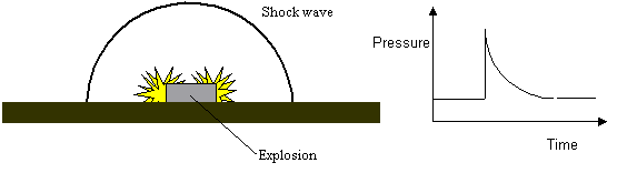
Blast WavesIf a strong gas explosion occurs inside a process area or in a compartment, the surrounding area will be subjected to blast waves. The magnitude of the blast wave will depend on:
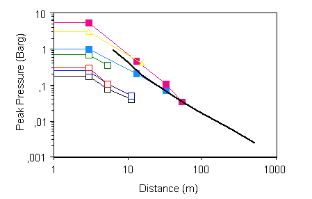
Figure 7.2 shows maximum explosion overpressures from various CMR experiments in a 50 m3 tube, a wedge-shaped vessel (results scaled to 50 m3) and a 50 m3 offshore module, together with the associated blast wave overpressure variation with distance. The horizontal part of the curves indicate the extent of the gas clouds before the explosions (actually the radius of a hemispherical cloud of the same volume as the experiment). No legend discriminating between the explosion vessels is given, since the gas volume and explosion overpressure are the important parameters here.
The results show that the blast wave from a gas explosion can cause high pressures far away from the area where the explosion actually takes place. In safety evaluation, free field blast must therefore be considered. In accident investigations evaluation of the free field blast from recorded damage is often used for evaluation of the source strength of the explosion. The objective of this chapter is: i) To describe the nature of a blast wave from a gas explosion.
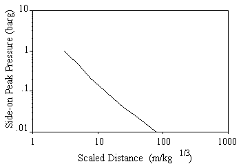
7.1 Scaling The blasts from detonations of high explosive charges, such as TNT, are fairly well documented. (Baker et al., 1983). The peak explosion pressure for blast waves from TNT explosions with charges ranging from 1 kg to 1000 kg, as function of distance R (from the centre of the charge) is shown in Figure 7.3.
These data can be scaled through a normalised length scale (Hopkinson scaling) R*
where R [m] is the distance from the centre of the explosive source and W[kg] is the mass of the explosive source. Figure 7.4 shows the same set of data as shown in Figure 7.3, but plotted versus the normalised length scale R*. Similar diagrams as Figure 7.4 also exist for duration, impulse and other blast parameters. These curves can be found in Baker et al. (1983).
7.2 TNT-Method The diagram for TNT detonations have been used for estimations of blasts from gas explosions, even though there are differences between the blasts from a gas explosion and a TNT-detonation (Shepherd et al., 1991, van den Berg, 1985). In a gas explosion the local pressure may reach values as high as a few bars. The blast pressure for TNT explosions is much higher close to the charge. Such near-field data are therefore irrelevant for gas explosions and it is recommended not to use TNT-data indicating pressures higher than 1 bar to estimate gas explosion blasts. The so-called TNT equivalence method has been widely used for gas explosions. The TNT equivalence method applies pressure-distance curves for TNT explosions to gas explosions and the equivalent TNT charge is estimated from the energy content in the exploding gas cloud. For typical hydrocarbons, such as methane, propane, butane etc., the heat of combustion is 10 times higher than the heat of reaction of TNT. The relation between the mass of hydrocarbons WHC and the equivalent TNT charge WTNT is then
where h is a yield factor (h = 3%-5%), based on experience, see Gugan, 1978. In the original TNT equivalence method, the mass of hydrocarbon WHC was based on the total mass released and the yield factor h. In order to estimate consequences of gas explosions, the geometrical conditions (i.e. confinement and obstructions) have to be taken into account. In the original TNT equivalence method, the geometrical conditions are not taken into account. The results from this type of analysis have therefore hardly any relevance and should in general not be used. The drawbacks of the TNT equivalence method can be listed as follows:
In order to take the geometrical effects into account in the TNT equivalence method, Harris and Wickens (1989) proposed to use a yield factor of 20% (h = 0.2) and the mass of hydrocarbon, WHC, contained in Stoichiometric proportions in any severely congested region of the plant. For natural gas the equivalent mass of TNT can be estimated from (assuming atmospheric pressure initially)
where V [m3] is the smaller of either the total volume of the congested region or the volume of the gas cloud. Equation 7.3 will also hold for most hydrocarbons, since the energy content per volume Stoichiometric mixture is approximately the same (~3.5MJ/m3). Figure 7.5 shows the results from a TNT equivalent analysis, as suggested by Harris and Wickens, in comparison with CMR's experimental results from 50 m3 tests.
As we can see from this figure there is fairly good agreement between the predicted values and the experimental values as long as the explosion pressure in the cloud is in a few bars range. Weak gas explosions (less than 0.5 bar) are not represented satisfactorily. This indicates that the TNT equivalence method can be useful as a rough approximation if one uses a yield factor of 20% and appropriate values for WHC or V. However, for explosion pressures below 1 bar, the TNT equivalence method will overestimate the blast. More sophisticated methods must therefore be applied for such cases.
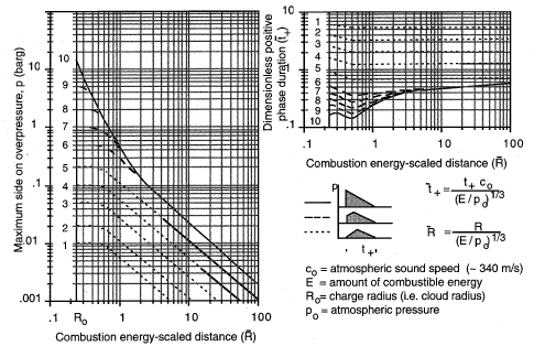
7.3 The Multi-Energy Method The multi-energy method (van den Berg, 1985) is a more sophisticated method than the TNT-equivalence method. It can estimate the blast from gas explosions with variable strength. The method is based on numerical simulation of a blast wave from a centrally ignited spherical cloud with constant velocity flames. By varying the flame velocity, a set of curves for different explosion strengths (i.e. explosion pressure inside the cloud) have been produced. Figure 7.6 shows the dimensionless curves that are used in the multi-energy method.
Figure 7.6 is in principle the same figure as the previous blast curves for TNT. For a detonating cloud, curve 10 can be used. For a deflagration (curves 1 to 9) we see that the pressure profile inside the cloud is not a shock wave followed by an expansion wave, but it can either be a shock wave followed by increasing pressure that drops off after the passage of the flame front or a sonic wave (i.e. gradually increasing pressure) that drops after the flame front. However, as a blast propagates away from the centre of the explosion, the gradient at the front will steepen and eventually become a shock wave, like the blast from a TNT charge. The difficult part of a multi-energy method analysis is to choose: i) The explosion pressure within the exploding gas cloud (i.e. the charge strength ii) The combustion energy, E, given the size of the gas cloud contributing to the blast (i.e. the charge size). The multi-energy method does not give any information about which explosion pressure (charge strength) to choose in a blast analysis. That information has to be found separately by using numerical simulations, experimental data or make a conservative assumption. The combustion energy, E, is also a parameter that is not straightforward to estimate. For a Stoichiometric hydrocarbon-air mixture of volume V, the combustion energy E can be estimated from
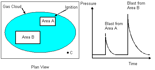
In an accidental explosion (deflagration), only the confined and/or congested areas will contribute to blast generation. Therefore only portions of the total cloud volume should be included in equation (7.4). Van den Berg (1985) indicates that the total volume of a confined and/or congested area should be used in equation (7.4). However, even such an approach can lead to conservative numbers and overestimate the blast in some situations. For instance in an explosion in a partly confined volume, the total volume will give conservative data, particularly in low pressure cases. During the explosion as the gas cloud burns the gas will expand and push the unburned gas outside the confinement. The gas that is pushed outside the confinement, will often not contribute significantly to the generation of the blast. Before we leave the multi-energy method there is one aspect of gas explosions that is discussed by van den Berg (1985) which should be mentioned. In a process area for instance, one large gas cloud can cause multiple blast waves. To illustrate this we include Figure 7.7. In this Figure we can see that the gas cloud covers two obstructed areas. Between these areas there is open space. If we assume that the cloud ignites in area A, we will first get an explosion in area A. If no transition to detonations occurs in area A, the flame velocity will drop when the flame propagates outside area A. In an open area, the flame velocity will be so slow that the pressure generation will be negligible. When the flame reaches area B, the flame will accelerate again and a new blast wave will be generated. If one monitors the pressure at location C, one will observe two blast waves passing.
This feature was also confirmed experimentally. Explosion propagation from one obstructed area into a second nearby obstructed area at various intervening distances shows deceleration of the flame upon propagating outside the first obstructed area and a re-acceleration within the second obstructed area (Figure 7.8) (van Wingerden, 1989).
7.4 Scaling of Experiments An alternative to the TNT-equivalence method and the multi-energy method is to scale experimental results. In Figure 7.2 some data from CMR experiments were presented. Based on these data and by applying scaling with dimensionless length scale, a set of curves for explosions with different strengths, for a 1000 m3 compartment, have been developed. The curves are shown in Figure 7.9.
For an explosion in a confinement of volume V the blast wave can be found simply by scaling the actual distance from the explosion centre R to an equivalent distance REq1000 and use that distance in Figure 7.9.
Results from such scaling are shown in Figure 7.10.
7.5 Numerical Methods Several advanced numerical codes for blast prediction exist. However, all these types of codes have limitations. They need either a predefined flame speed or explosion pressure (i.e. they cannot estimate source term) or they require computers of an order of magnitude larger than we have today to handle both flame propagation and blast propagation. Savvides and Tam (1991) have compared FLACS results with results from TNT equivalence and multi-energy methods. It was found that in the test cases used, the high overpressure was created in localised pockets within the plant, where the density of equipment was high. They observed that the overpressure decayed rapidly in open space. The conclusions were that a numerical simulation model like FLACS provides much more information than the simpler models, but the requirement for computer time is high for process plants. They foresee that such simulations will become a routine task in assessing explosion hazards. At CMR the FLACS-3D code has been used for combined explosion and blast simulations even though the main use of FLACS is in simulating gas explosions only. The main difference between the two applications is that blast simulations are usually performed on a large calculation domain, where the explosion takes place in a smaller part of this domain. Due to limitations in computer capacity larger control volumes must be used, which may not be compatible with the fact that in onshore plants localised explosions can be very important. To handle localised explosion in the simulations, small control volumes are needed. However, for local explosions of a given source strength, FLACS is still suited to predict blast decay in congested or semi-confined surroundings of the exploding gas cloud. Figures 7.10 and 7.11 compare examples of blast decay simulations using FLACS in local explosions in a process plant with scaled experimental results (using equation 7.5) for two clouds of 20 m3 and 600 m3 respectively. The scaled experimental results are based on one test in CMR's 50 m3 model of an offshore module (Figure 7.11 only, see section 5.6) and on two tests in the 10 m long tube (see section 5.3), producing maximum pressures inside the gas cloud of 0.2, 1 and 6 barg respectively. The FLACS simulations generate 0.3 bar overpressure in the 20 m3 cloud and 5-6 bar overpressure in the 600 m3 cloud. The simulated pressure decay outside the gas clouds shows a behaviour very similar to the experimental results. The observed deviations may be due to differences in congestion outside the exploding gas cloud.
The vertical lines in Figures 7.11 and 7.12 show the radius of equivalent, hemispherical gas clouds of volumes 20 m3 and 600 m3 respectively.
7.6 Reflection of Free Field Blast Waves The loading on a construction hit by a blast wave is a rather complex phenomenon. (Baker et al.(1983). When a free field blast wave runs into an object like a building, the wave will be reflected. Figure 7.13 shows how a shock wave is reflected off a building. Due to reflection and diffraction, the wave loading on the walls and the roof will differ. The maximum loading will be on the wall facing the explosion. At this wall the shock wave will be reflected and the pressure will typically increase by a factor of 2. (Depends on shock strength.). When the shock wave propagates in a free field, the gas behind the shock wave will have a velocity in the same direction as the wave propagates. When the shock wave hits the wall, the gas must stop and the dynamic pressure (i.e. 0.5 ru2) is transformed to pressure. This is in principle why the pressure increases due to blast wave reflection. On the opposite wall (see Figure 7.13) the shock wave will be diffracted, and that will reduce the pressure load on the building.
7.7 Guidelines for Blast Waves
注意:本栏目所有书籍均来至于网络,如果其中涉及了您的版权,请及时联系我们,我们在核实后将在第一时间予以删除!
|